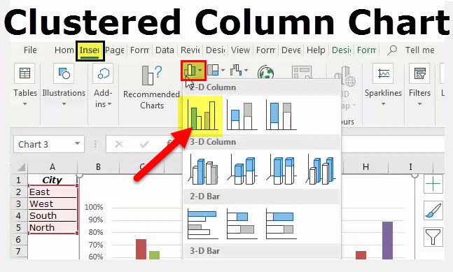
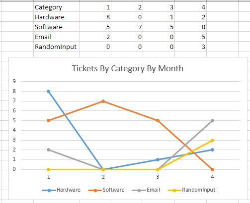
Excel Pivot Chart Trendline Across Multiple Columns – You may create a multiplication chart in Stand out by using a format. You will discover a number of samples of web templates and learn how to structure your multiplication graph or chart using them. Here are a few tips and tricks to make a multiplication graph or chart. After you have a design, all you need to do is duplicate the solution and paste it in the new cell. You can then use this formula to increase several amounts by an additional established. Excel Pivot Chart Trendline Across Multiple Columns.
Multiplication kitchen table format
You may want to learn how to write a simple formula if you are in the need to create a multiplication table. First, you should locking mechanism row one of several header line, then grow the quantity on row A by cellular B. An additional way to create a multiplication kitchen table is to apply merged recommendations. In this instance, you would probably enter $A2 into line A and B$1 into row B. The end result is really a multiplication table with a solution that really works for columns and rows.
If you are using an Excel program, you can use the multiplication table template to create your table. Just open the spreadsheet together with your multiplication table change and template the brand towards the student’s brand. You can also modify the sheet to suit your individual requirements. There is an method to affect the shade of the cells to improve the look of the multiplication table, way too. Then, you are able to alter the range of multiples to suit your needs.
Developing a multiplication graph in Stand out
When you’re utilizing multiplication dinner table computer software, it is possible to produce a easy multiplication kitchen table in Shine. Simply produce a sheet with rows and columns numbered in one to 40. In which the rows and columns intersect will be the answer. For example, if a row has a digit of three, and a column has a digit of five, then the answer is three times five. The same thing goes for the opposite.
Initially, you can enter the figures that you need to increase. If you need to multiply two digits by three, you can type a formula for each number in cell A1, for example. To produce the numbers larger sized, pick the tissues at A1 and A8, after which click the proper arrow to select a variety of cellular material. After that you can sort the multiplication formula inside the tissues in the other columns and rows.
Gallery of Excel Pivot Chart Trendline Across Multiple Columns